
CPPGPGPU Comes with a series of examples. The general use of CPPGPGPU is to simply duplicate an existing example that does something close to what you want to do, then modify the example to your needs, rename it and you have yourself a program. These examples cover a wide variety of applications and ideas that one could utilize and work on. If you come up with a cool application yourself, you are strongly encouraged to contact the lead developer (CNLohr) to commit your example to our project.
Many of these examples are not in fact GPGPU. CPPGPGPU caters to GPGPU but does not limit itself to strict GPGPU applications. For instance the noise and Julia Set shaders have virtually nothing to do with GPGPU.
Examples include each of the following:
General notes regarding these projects:
These examples come with images generated by Graphviz that aide in the explanation of what's going on. Because of the large size of the image, it's suggested you view this page with a resolution of 1024x768 or greater. The source for the graphviz files can be found in the graphviz/ folder. For reference, they were generated using the following command:
cat {file}.png | dot -Tpng > {file}.png
The below (with the exception of scenegraph) use the following legend when describing all nodes. The name in the node normally refers to the variable name that the node has in the main.cpp file. Inside each large square is the general operation being performed. The arrows inside the square indicate order of information flow. The arrows pointing from square to square indicate the order in which everything gets executed.
One common theme throughout the projects is the copy stage. The copy stage is a common theme in these applications. It is possible to essentially double-buffer textures, but since most of the time, we are performing a tremendous amount of work on these textures, a copy step does not raise much of a slowdown. If you are doing something that you really need to get serious speed with, you should avoid the copy stage by rotating your textures. It is imperative that you have two textures! You cannot output to a texture you are inputting from, this will cause very strange results and will many times produce complete failure of operations.
All results in FPS. XXX indicates example will not operate on hardware correctly.
| Demo | GF 6600 Go (lin) | GF 7600 GS (win) | GF 7600 GS (lin) | GF 8600 GT(lin) |
| Andrewmath (w/ transfer) | 41 | 70 | 69 | 154 |
| Andrewmath (w/o transfer) | 52 | 110 | 123 | 195 |
| Clothsim | 490 | 775 | 669 | 2093 |
| Jiggily | 680 | 750 | 750 | 2480 |
| Julia | 24-298 | 64-494 | 65-492 | 303-1387 |
| Mandelbrot | 30 | 89 | 89 | 478 |
| Partic | 96 | 186 | 198 | 349 |
| Ballscene | 6-11 | 16-30 | 17-30 | 43-84 |
| Rnoise | 144 | 295 | 312 | 810 |
| Multipass | 47 | 149 | 147 | 299 |
| Scenetest | 170 | 272 | 308 | 525 |
Andrewmath was originally going to be a particle wave physics simulation, however it ended up being simplified into a general 2D wave simulation. In the example provided, it is performed on a 256x256 set of cells with sWork shader.
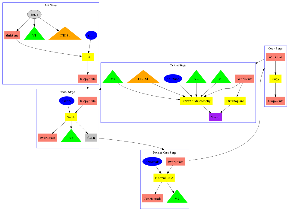
In the initial setup steps of andrewmath, V1 is simply loaded with locational information for the map of all verticies. This allows us to know, in the SSurface shader what the location is for our current vertex on the XY plane. ITRIS1 is loaded with geometry information, a series of 6*total points indices, effectively making a grid of triangles for visualization. tInitState is loaded with the initial state of the fluid. This state is a semi-oval in the middle, that is extremely tall. Additionally, tInitState[3] is loaded off disk (andrew.ppm). The InitData() function gets called whenever the user presses the 'a' key on the keyboard.
In the work stage, tWorkState is designated as the output for the sWork shader. Inside the shader, it has access to multiple CopyState buffers. The very first of the tWorkState buffers are both streamed into vertex data, as well as read back to the CPU every cycle. The fData step can be ignored.
Inside the sWork shader is the workload for the wave physics occur. This shader is read using Work.frag/.vert. The primary work is done in the fragment program. The physics is as simple as taking the laplacian of the surrounding points and modifying the velocity (delta-Z) accordingly. Once the velocity is changed accordingly, the value simply changed based on this velocity, +/- potential information, provided at init by Texture3.
The normal stage is very straightforward. It only looks at the values at each point surrounding the point it's attempting to find the normal for. Simply looking at the delta-z in the y direction and the delta-z in the x direction provides all the information necessary to find the normal at that point. This data is both outputted to the TexNormals as well as to V2 so that it can be used in the Output Stage's SSurface vertex shader.
The output stage has access to almost everything. Since we were careful to pack our data into vertex buffer objects, V1-V3, we do not need to make any texture lookups in the vertex shaders, instead the normal, altitude and location of each one of the 256 cells is given to us. The work state is provided along with just in case the SSurface would at some future time want to have access to altitude information from its neighbors.

Andrewmath code can be viewed anonymously via SF.net ViewSVN here.
Clothsim is a very basic cloth simulation using 64x64 points. Each point is connected to each of the points around it (one in each direction) by a mass spring. Each one of these mass springs attempts to maintain the distance from it to its neighbor. If there is a stress, pulling it in one direction, it will apply a force in the opposite direction in order to try to maintain its general shape. Once gravity is applied, it's trivial to do all sorts of "fun" things with this cloth simulation. You can see an earlier version of this cloth simulation on youtube here.

The set up for the cloth simulation is a little simpler than that for the wave simulation. All that's necessary is to set the values of all the coordinates back to the original starting location. Since each texel in TexCpy[0]/TexOut[0] corresponds to the x/y/z location of the cell, set up for the absolute location isn't even that hard.
The big difference between this and the wave simulation is that in this one, TexCpy[0]/TexOut[0] and TexCpy[1]/TexOut[1] correspond to absolute 3D locations and 3D velocities. This makes normal calculation a little harder, and everything else a little easier.
In the SDoCalc shader (Corresponding to DoCalc.vert/DoCalc.frag), basic physics rules are performed, including the application of gravity and integration of position with respect to velocity. All shapes that the cloth is falling onto are implicitly described by basic math operations. For instance, the sphere at -.8,.8,1. is detected simply by the clause ( distance( vec3( -.8,0.8,1.), pos.xyz ) < .2 ) where pos is the position of {this} point on the cloth. At a later point in the shader, the actual spring physics is performed comparing the position of pos to all of its neibhors and applying forces accordingly.
The output for this system is extremely basic and parallels the wave simulation.

Clothsim code can be viewed anonymously via SF.net ViewSVN here.
Jiggily is a brief exploration of something very similar to the clothsim, except with one major difference. It can be applied on an arbitrary triangulated mesh. The adjacency information is stored in the CrosReference texture. This allows mesh deformation, with accurate normal reconstruction to be performed on the GPU entirely, without any data being sent back to the CPU.

The Init stage is slightly more complex than either of the previous two demos. It is necessary for all geometry information, indices, and V1 to be loaded from a mesh, instead of synthesized. OPos, the original position of all items must be stored as well, so distance comparisons may be performed later. The minor innovation here comes in with the CrossReference texture. This texture is 4 times wider and 4 times higher than the OPos texture. That is because for each pixel in OPos, there are 16 texels that describe the geometry. A total of eight triangles may be connected to any vertex and this system will not break. It allows very fast indexing in the SDoCalc and SNormal fragment shaders so any one vertex may be able to find all edge information necessary for doing normal reconstruction or attempting to reform the mesh.
The work stage is modified, but the details there are un-important. Instead of the work stage being split up into a work and a normal stage, both are performed at the same stage, but sequentially. First the Work, then the Normals.
Since all of the vertices are slammed into the TexCpy and OPos textures, running a fragment shader on this data provides a one-to-one correspondence to the vertex information, allowing the vertex information to be modified from frame-to-frame, with texture lookups and all operations normally useful in a fragment shader, while the output is sent directly to a vertex shader.
The SDoCalc shader only attempts to maintain distance on all of its vertices. Making a large mass spring system. This allows the mesh to rotate freely, without being restricted to its original rotational form. This poses a problem, that large shapes can crunch up, as this example does after several minutes of running.
The SNormal shader can simply look up in a texture where it's position in 3D space is, then look up in the CrossReference texture for the vertices applicable to its first connected triangle, and the second and so on. A normal triangle normalization process is run and the result normalized per-pixel. Note that the work for finding a triangle's normal is performed three times as much as it needs to. Because of the system we're doing this with, in order to do per-triangle normals and then per-vertex normals, a new stage and the per-triangle code would need a new crossreference texture to know what vertices belonged to it. This was found to be too much work, and a compromise here was reached.
The output stage very closely resembles the normal output stages for the previous projects. Note that the V1/V2/V3 information is swapped around a little in this project, but not to any serious level.
The output here is a geosphere (level 2) It's colored with the normals being applied for verification that the normals do change based on the shape and rotation of the object.

Jiggily code can be viewed anonymously via SF.net ViewSVN here.

There isn't any real set up for this app, it's more or less just a shader being applied to a square that's the size of the screen. The code itself simply implements a loop that gets executed a maximum of 32 times. In each loop, it performs 4 iterations of the complex function. While somewhat confusing, all of the (numbers) used in this shader are complex numbers, easily representable by a vec2. Functions like length(), + and - operate on the complex representation exactly as you would expect it to. Things don't get harry until you try squaring the numbers.
Juliaset code can be viewed anonymously via SF.net ViewSVN here.

Mandelbrotset code can be viewed anonymously via SF.net ViewSVN here.
Multipass is an example of a multi-pass scene being rendered using cppgpgpu. This is also not very GPGPU related whatsoever. It implements some filters, and floating point textures. It was actually done as an assignment for a class I had. If you want to read more about this example, please download the pdf here.

Multipass code can be viewed anonymously via SF.net ViewSVN here.
Partic is a basic particle system that simulates 65,536 particles (one particle per texel on a 256x256 image) falling through a bowl with a hole at the bottom.

It's strongly encouraged that you read the general flow of what's going on from the cloth sim, as it's extremely similar. The only notable difference is the fact that this uses DrawGeometry() instead of DrawSolidGeometry().
This is actually a much better starting point if you want to start playing around with fragment shaders that control vertex buffer objects. It uses a very simple implicitly defined shape and provides very basic rules for all of the particles in the system.
Additionally, this is an example of when the debugging square at the bottom can come in very handy, to figure out where all your particles went.

Partic code can be viewed anonymously via SF.net ViewSVN here.
Ballscene is an example of ray tracing on the GPU. This is a very basic scene with a total of eight reflective balls, two lights and a normal-mapped ground in motion. Like classic ray tracing, this tests every single ray against every single other object, and it tests all secondary rays against every other object.

The actual shader packs all of the sphere information into separate vec4's that are hard coded in the shader. In solving the basic sphere-ray intersection, some components can fall out as a fixed function of the sphere and of the ray. These terms (The A and C terms) are stored so that they do not have to get recomputed for every ray-sphere hit check.
When colliding against every sphere, the test first does a determinant to check if it hit the sphere at all. If so, depth information is calculated, otherwise it moves on. In the event of shadow ray checking, this process can be sped up immensely.
When colliding with the ground, it is trivial to do a ground check by using a ray/plane intersection check, and then applying additional conditions to the hit test. The normal is trivially found by using the world coordinates of the hit as texture coordinates.
The primary loop is very straightforward and can loop up to a maximum of five times for secondary rays. Much more than this and the "interactive" features of this project become startlingly less interactive.
This is a screen shot of the newest version, an older version video can be found on youtube here.

Ballscene code can be viewed anonymously via SF.net ViewSVN here.
WARNING: This implementation of Perlin noise is incorrect. It will be investigated.
This is a basic demo of some perlin noise code I threw together. By default, it uses 3D perlin noise to add perturbation to a simple wooden log shader. Like several of the other projects, this also does not have very many GPGPU applications. Because this one is questionable, a detailed description will not be coevered.


RNoise code can be viewed anonymously via SF.net ViewSVN here.
Scenetest is a test of the Scene Graph functionality, available in the Extras/ folder in cppgpgpu. The idea is that it allows you to take a much more object oriented approach to performing the tasks you would normally use cppgpgpu for. This may get updated in the future with a more comprehensive set of tools, but as of now this is what you get.
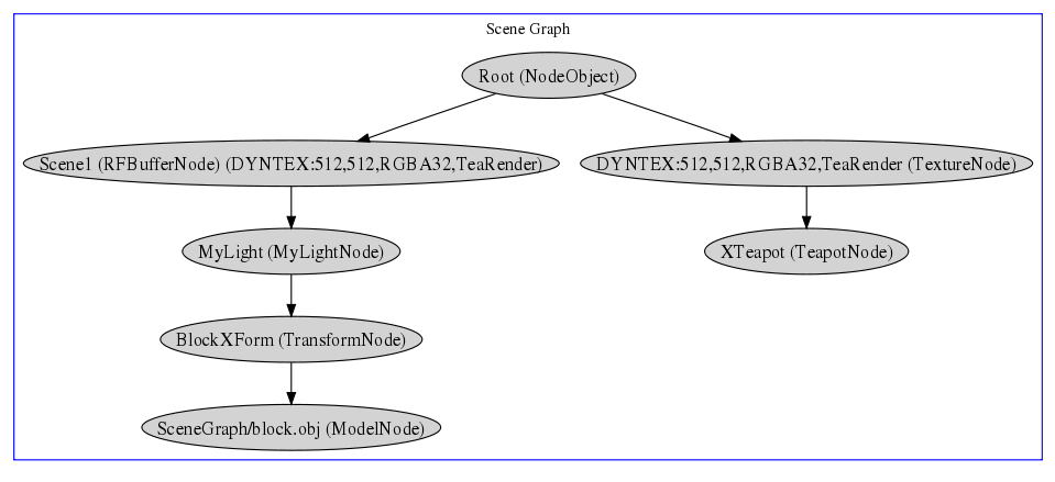
In this system, we have the following code:
The idea is that each node can have children added to it. So, for the lefthand side of the tree, we populate it with a render/frame buffer node called "Scene1" this causes everything underneath of it to be rendered to another target (wich is configured later on. A lighting node and the transform node get applied to the block model that gets rendered to the framebuffer. On the other side of the tree, we apply a texture node and apply that texture to a teapot model. The texture that is being used is used to configure the render/frame buffer.

Scenegraph Test code can be viewed anonymously via SF.net ViewSVN here.